Code
%pip install -q -e ..Note: you may need to restart the kernel to use updated packages.This project examines habitat suitability for Blue Stem in the Buffalo Gap and Oglala National Grasslands. See also PAD-US.
These contiguous grasslands are located in Oceti Sakowin Oyate, also known as the Lakota Nation or Great Sioux Nation, and in the US states of South Dakota and Nebraska. For more information see Oceti Sakowin Essential Understandings & Standards.
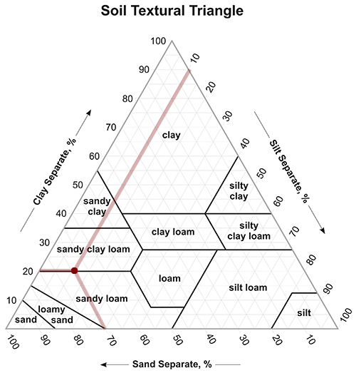
Blue Stem, according to Greg, “need well-drained, nutrient-rich soils. The best soil types for this grass are sandy loam or loamy soil, which provide the right balance of drainage and nutrients. Aim for an organic matter content of 5-10%. This range is crucial for optimal growth, as it enhances soil fertility and structure. The ideal pH range for Big Bluestem is between 6.0 and 7.0. This slightly acidic to neutral pH is essential for nutrient availability, ensuring your plants can absorb what they need to thrive.”
Gardners.com has a soil simplex figure, which puts sandy loam and loamy sand at 50-85% sand.
I could not find information on slope or aspect but I have seen blue stem on flat areas and slopes.
First visit USFS Geospatial Data Discovery: National Grassland Units (Feature Layer) and manually download GeoJSON file from DataSet into directory ~/earth-analytics/data/habitat (see create_data_dir() below). A GeoDataFrame buffalo_gdf is created and stored for later retrieval to save time. The plot_redline() function is from landmapyr.redline module to visualize.
%pip install -q -e ..Note: you may need to restart the kernel to use updated packages.import geopandas as gpd # read geojson file into gdf
from landmapyr.initial import create_data_dir # create (or retrieve) data directory
from landmapyr.plots import plot_gdf_state # plot gdf with state overlay%store -r buffalo_gdf
try:
buffalo_gdf
except NameError:
data_dir = create_data_dir('habitat')
# Read all grasslands GeoJSON into `grassland_gdf`.
grassland_url = f"{data_dir}/National_Grassland_Units_(Feature_Layer).geojson"
grassland_gdf = gpd.read_file(grassland_url)
# Subset to desired locations.
buffalo_gdf = grassland_gdf.loc[grassland_gdf['GRASSLANDNAME'].isin(
["Buffalo Gap National Grassland", "Oglala National Grassland"])]
%store buffalo_gdf
print("buffalo_gdf created and stored")
else:
print("buffalo_gdf retrieved from StoreMagic")buffalo_gdf retrieved from StoreMagicBlack line separates South Dakota from Nebraska; red line outlines part of Pine Ridge Reservation.
plot_gdf_state(buffalo_gdf, aiannh=True)
Download soil raster layer for sand covering study area envelope using the POLARIS dataset. Considering sand percentage mean. POLARIS data are available at 6 depths, and Bluestem has roots down to 5 feet (150 cm), which is the lowest strata measured (100-200 cm). Data in the sand 100-200 cm directory are saved as separate tif files by longitude. Buffalo Gap National Grassland is at (centroid) 43.4375° N, 103.0505° W, while Oglala National Grassland is at 42.9404° N, 103.5900° W. Below we use the .total_bounds extension on buffalo_gdf with the merge_soil() function in the landmapyr.polaris module to automate finding bounds.
Get and show mean of sand at depth 100-200m with functions
buffalo_da = merge_soil(buffalo_gdf, "sand", "mean", "100_200")plot_gdf_da(buffalo_gdf, buffalo_da)from landmapyr.polaris import merge_soil # merge soil data from GDF
from landmapyr.plots import plot_gdf_da # plot GDF over DAMerge soil tiles to create buffalo_da.
print(buffalo_gdf.total_bounds)
%store -r buffalo_da
try:
buffalo_da
except NameError:
buffalo_da = merge_soil(buffalo_gdf)
print("buffalo_da merged soil from buffalo_gdf and stored")
else:
print("buffalo_da soil merge retrieved")[-104.05473027 42.74093601 -101.47233564 43.99459902]
buffalo_da soil merge retrievedbuffalo_gdf['color'] = ['white','red']
plot_gdf_da(buffalo_gdf, buffalo_da, cmap='viridis')
Project precipation pr under representative concentration pathway scenarios rcp45 and rcp85 for years 2026-2030.
from landmapyr.thredds import process_maca, maca_yearinfo_df, maca_da = process_maca({'buffalo': buffalo_gdf})
info_dfYears: 2026 2030| site_name | scenario | climate | |
|---|---|---|---|
| 0 | buffalo | pr | rcp85 |
| 1 | buffalo | pr | rcp45 |
maca_2027_year_da = maca_year(maca_da[0], 2027) # 0 = `rcp85`, 1 = `rcp45`
plot_gdf_da(buffalo_gdf, maca_2027_year_da)
Repeat for rcp45. Make nice plot pair. Will need to modify plot_gdf_da() to return object rather than create plot. This probably has some subtleties.
import earthaccess
from landmapyr.srtm import srtm_download, srtm_slopeproject_dir = create_data_dir('habitat')
elevation_dir = create_data_dir('habitat/srtm')
elevation_dir'/Users/brianyandell/earth-analytics/data/habitat/srtm'earthaccess.login()
datasets = earthaccess.search_datasets(keyword='SRTM DEM', count=11)
for dataset in datasets:
print(dataset['umm']['ShortName'], dataset['umm']['EntryTitle']) # want 'umn'
# want SRTMGL1? 1 arc second = 30m (also, 3, 30 arc second)NASADEM_SHHP NASADEM SRTM-only Height and Height Precision Mosaic Global 1 arc second V001
NASADEM_SIM NASADEM SRTM Image Mosaic Global 1 arc second V001
NASADEM_SSP NASADEM SRTM Subswath Global 1 arc second V001
C_Pools_Fluxes_CONUS_1837 CMS: Terrestrial Carbon Stocks, Emissions, and Fluxes for Conterminous US, 2001-2016
SRTMGL1 NASA Shuttle Radar Topography Mission Global 1 arc second V003
GEDI02_B GEDI L2B Canopy Cover and Vertical Profile Metrics Data Global Footprint Level V002
GEDI01_B GEDI L1B Geolocated Waveform Data Global Footprint Level V002
NASADEM_HGT NASADEM Merged DEM Global 1 arc second V001
SRTMGL3 NASA Shuttle Radar Topography Mission Global 3 arc second V003
AST14DEM ASTER Digital Elevation Model V004
NASADEM_NC NASADEM Merged DEM Global 1 arc second nc V001srtm_da = srtm_download(buffalo_gdf, elevation_dir, 0.1)
plot_gdf_da(buffalo_gdf, srtm_da, cmap='terrain')
slope_da = srtm_slope(srtm_da)
plot_gdf_da(buffalo_gdf, slope_da, cmap='terrain')/users/brianyandell/miniconda3/envs/earth-analytics-python/lib/python3.11/site-packages/dask/dataframe/__init__.py:49: FutureWarning:
Dask dataframe query planning is disabled because dask-expr is not installed.
You can install it with `pip install dask[dataframe]` or `conda install dask`.
This will raise in a future version.
warnings.warn(msg, FutureWarning)
Alternate plot only inside grasslands. Want to smooth over buffalo_gdf to fill in internal holes.
import matplotlib.pyplot as plt # Overlay raster and vector data
slope_clip_da = slope_da.rio.clip(buffalo_gdf.geometry)
slope_clip_da.plot(cmap='terrain')
#buffalo_gdf.boundary.plot(ax=plt.gca(), color = "black", linewidth=0.5)
plt.show()
See 3_harmonize.
buffalo_sand_da = buffalo_da.rio.reproject_match(slope_da)
maca_2027_da = maca_2027_year_da.rio.reproject_match(slope_da)See
Currently using python 3.11.10 with the earth-analytics-python environment. Using StoreMagic to store and retrieve intermediate calculations. Markdown rendered with quarto render buffalo.qmd -t markdown. Code chunks are specific to this project (using name buffalo) but use generic functions from the landmapyr module.
The project compares
rcp45 (4.5 = current) and rcp85 (8.5 = worse case)The pseudocode below relies on routines I developed with guidance from course instructors and fellow students, organized with modules and their functions in the package landmapyr as DRY code. Workflows cited above have more detail on use and initial plots.
buffalo_gdf is created in step 0 and then stored for later retrieval.
grassland_gdf = gpd.read_file(grassland_url)buffalo_gdf = grassland_gdf.loc[...]plot_redline(buffalo_gdf)mean of sand at depth 100-200m is created (ignoring buffer of 0.1) with functions
buffalo_da = merge_soil(buffalo_gdf, "sand", "mean", "100_200")plot_gdf_da(buffalo_gdf, buffalo_da)pr
rcp45, rcp85
info_df, maca_da = process_maca({'buffalo': buffalo_gdf}, ['pr'], ['rcp85', 'rcp45'], [2026])maca_2027_year_da = maca_year(maca_da[0], 2027) # 0 = rcp85, 1 = rcp45plot_gdf_da(buffalo_gdf, maca_2027_year_da)slope
srtm_da = srtm_download(buffalo_gdf, elevation_dir, 0.1)slope_da = srtm_slope(srtm_da)plot_gdf_da(buffalo_gdf, slope_da)buffalo_sand_da = buffalo_da.rio.reproject_match(slope_da)maca_2027_da = maca_2027_year_da.rio.reproject_match(slope_da)ramp_logic(maca_2027_da, (500, 550), (700, 750)).plot()ramp_logic(buffalo_sand_da, (50, 60), (80, 90)).plot()ramp_logic(slope_da, (0, 5), (15, 20)).plot()Workflow details were developed in separate jupyter notebooks. Working documents that contribute to this workflow are as follows.
Download climate raster layers covering study area envelope, including:
http://thredds.northwestknowledge.net:8080/thredds/dodsC/MACAV2/BNU-ESM/macav2metdata_pr_BNU-ESM_r1i1p1_rcp85_2026_2030_CONUS_monthly.nc (strip off trailing .html)_pr_) with OPENDAP
Download elevation raster layer covering your study area envelope. Consider slope or aspect to use in your model. Probably use the xarray-spatial library, which is available in the latest earth-analytics-python environment (but will need to be installed/updated if you are working on your own machine). Note that calculated slope may not be correct if you are using a CRS with units of degrees; re-project into a coordinate system with units of meters, such as the appropriate UTM Zone.
Specifically, X,Y are lon,lat in degrees, while Z (height) is in meters. Need to reproject into UTM with meters, which meanes we have to find the UTM Zone. Need to find our area. The UTM Zone Finder shows that we are in UTM Zone 13 (and actually 13N north). We need the projection (EPSG) for UTM zone 13N, which is EPSG:32613 by looking at https://epsg.io.
Make sure to reproject so grids for all layers match up. Check out the ds.rio.reproject_match() method from rioxarray.
To train a fuzzy logic habitat suitability model:
References