Code
%pip install -q -e ..Left to do:
reproject code in place.Python code setup:
%pip install -q -e ..import pandas as pd
import geopandas as gpd # read geojson file into gdf
import matplotlib.pyplot as plt # Overlay raster and vector data
import xarray as xr
from landmapyr.initial import create_data_dir # create (or retrieve) data directory
from landmapyr.plots import plot_gdf_state # plot gdf with state overlay
from landmapyr.plots import plot_gdf_da # plot GDF over DA
from landmapyr.plots import plot_das # plot DAs in rows
from landmapyr.process import da_combine
from landmapyr.polaris import merge_soil # merge soil data from GDF
from landmapyr.srtm import srtm_download, srtm_slope # process SRTM data
from landmapyr.thredds import process_maca, maca_year # process MACA THREDDS
from landmapyr.explore import ramp_logic # ramp for fuzzy logicOur changing climate is changing where key grassland species can live, and grassland management and restoration practices will need to take this into account (Kane et al. 2017).
In this coding challenge, create a habitat suitability model for a species of your choice that lives in the continental United States (CONUS). We have this limitation because the downscaled climate data we suggest, the MACAv2 dataset, is only available in CONUS. If you find other downscaled climate data at an appropriate resolution you are welcome to choose a different study area. If you don’t have anything in mind, you can take a look at Sorghastrum nutans, a grass native to North America. In the past 50 years, its range has moved northward (GBIF S. nutans).
Your suitability assessment will be based on combining multiple data layers related to soil, topography, and climate. You will also need to create a modular, reproducible, workflow using functions and loops. To do this effectively, we recommend planning your code out in advance using a technique such as pseudocode outline or a flow diagram. We recommend planning each of the blocks below out into multiple steps. It is unnecessary to write a step for every line of code unles you find that useful. As a rule of thumb, aim for 2-5 line code chuck for major structure steps.
Before you begin coding, you will need to design your study.
Reflect and Respond: What question do you hope to answer about potential future changes in habitat suitability?
YOUR QUESTION HERE
Select the species you want to study, and research it’s habitat parameters in scientific studies or other reliable sources. You will want to look for reviews or overviews of the data, since an individual study may not have the breadth needed for this purpose. In the US, the National Resource Conservation Service can have helpful fact sheets about different species. University Extension programs are also good resources for summaries.
Based on your research, select soil, topographic, and climate variables that you can use to determine if a particular location and time period is a suitable habitat for your species.
Reflect and Respond: Write a description of your species. What habitat is it found in? What is its geographic range? What, if any, are conservation threats to the species? What data will shed the most light on habitat suitability for this species?
YOUR SPECIES DESCRIPTION HERE
Big bluestem is a warm-season grass native to the eastern two thirds of the United States from the mid-western short grass prairies to the coastal plain. It grows to 6 to 8 feet with short and scaly rhizomes and leaves that vary from light yellow-green to burgundy. The seed head is coarse and not fluffy, typically with three spikelets looking like a turkey foot.
Below are two pictures of me and my (leashed) dog, Kylie, on a walk in Prairie Moraine County Park (Dane Co, WI) surrounded by bluestem. We were walking on the Ice Age National Scenic Trail Corridor just north of the dog part. The Ice Age Trail is a 1000-mile system that comprises a unique boundary separating the glaciated and “driftless” regions across the state of Wisconsin. Bluestem is found along much of this trail system.


Bluestem can tolerate a wide variety of well-drained soils and typically does well on low fertility sites. Big blue is commonly used in erosion control plantings. While it may be slow to get started, it eventually provides excellent stability for sandy areas. It is also a good native choice for grazing forage and provides excellent wildlife habitat. Bobwhite quail and other ground-nesting birds use this clump-forming grass for nesting and forage cover. In the longleaf pine ecosystem, the perennial big bluestem contributes to the fine flashy fuel needed for the maintenance of the ecosystem.
Bluestem can be used in the restoration of native vegetation in agricultural or pasture areas. It is adapted to conventional tillage or native seed no-till drill. Seeding rate for big bluestem ranges from 4 to 12 pounds per acre, lower for wildlife (quail) habitat establishment. Local ecotypes are best when restoring native vegetation areas.
Bluestem grasses have root systems that reach significant depths. In Buffalo Gap National Grassland, these grasses typically develop roots that extend up to 5 feet deep. This deep root system helps them access water and nutrients from deeper soil layers, making them resilient in the semi-arid conditions of the grassland.
Blue Stem, according to Greg, “need well-drained, nutrient-rich soils. The best soil types for this grass are sandy loam or loamy soil, which provide the right balance of drainage and nutrients. Aim for an organic matter content of 5-10%. This range is crucial for optimal growth, as it enhances soil fertility and structure. The ideal pH range for Big Bluestem is between 6.0 and 7.0. This slightly acidic to neutral pH is essential for nutrient availability, ensuring your plants can absorb what they need to thrive.”
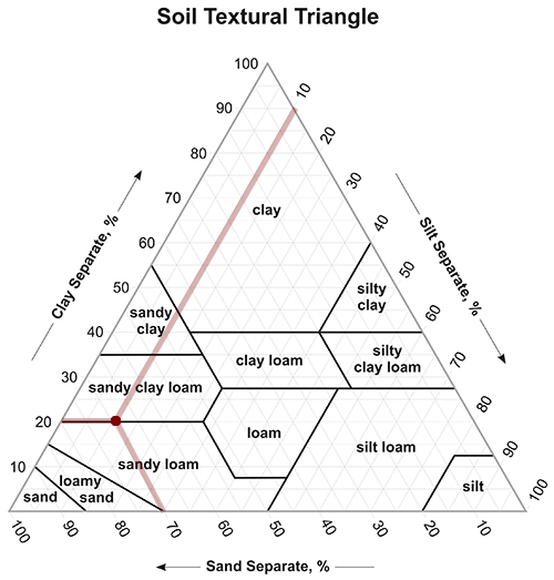
Gardners.com has a soil simplex figure, which puts sandy loam and loamy sand at 50-85% sand.
According to the USDA Natural Resources Convervations Service: Plant Guide: Little Bluestem “is a tallgrass prairie increaser and mixed prairie decreaser. Little bluestem typically occurs on dry upland sites, especially on ridges, hilltops, and steep slopes. It also occurs on limey sub-irrigated sites and in prairie fens. It is found in areas receiving 10 to 60 inches of mean annual precipitation and plant hardiness zones 3 to 9.” Plant profile page.
Big Bluestem “is climatically adapted throughout the Midwest and Northeast on moderately well drained through excessively well drained soils. It is adapted to a range of other soil limitations such as shallow depth, low pH, and low fertility.” Plant profile page.
While I could use GBIF to find crowd-sourced records, these two species are widely found across North America. For more on using GBIF with Python, see
gbif.py module)Select at least two site to study, such as two of the U.S. National Grasslands. You can download the National Grassland Units and select your study sites. Generate a site map for each location.
When selecting your sites, you might want to look for places that are marginally habitable for this species, since those locations will be most likely to show changes due to climate.
Reflect and Respond: Write a site description for each of your sites, or for all of your sites as a group if you have chosen a large number of linked sites. What differences or trends do you expect to see among your sites?
This project examines habitat suitability for Blue Stem in the Buffalo Gap and Oglala National Grasslands.
Resources:
These contiguous grasslands are located in Oceti Sakowin Oyate, also known as the Lakota Nation or Great Sioux Nation, and in the US states of South Dakota and Nebraska. For more information see Oceti Sakowin Essential Understandings & Standards.
Get grassland GeoDataFrames and focus on desired sites. Pseudocode:
data_dir = create_data_dir('habitat')
grassland_url = f"{data_dir}/National_Grassland_Units_(Feature_Layer).geojson"
grassland_gdf = gpd.read_file(grassland_url)
buffalo_gdf = grassland_gdf.loc[grassland_gdf['GRASSLANDNAME'].isin(
["Buffalo Gap National Grassland", "Oglala National Grassland"])]
plot_gdf_state(buffalo_gdf, aiannh=True)Python code detail:
%store -r buffalo_gdf
try:
buffalo_gdf
except NameError:
data_dir = create_data_dir('habitat')
# Read all grasslands GeoJSON into `grassland_gdf`.
grassland_url = f"{data_dir}/National_Grassland_Units_(Feature_Layer).geojson"
grassland_gdf = gpd.read_file(grassland_url)
# Subset to desired locations.
buffalo_gdf = grassland_gdf.loc[grassland_gdf['GRASSLANDNAME'].isin(
["Buffalo Gap National Grassland", "Oglala National Grassland"])]
%store buffalo_gdf
print("buffalo_gdf created and stored")
else:
print("buffalo_gdf retrieved from StoreMagic")buffalo_gdf retrieved from StoreMagicBlack line separates South Dakota from Nebraska; red line outlines part of Pine Ridge Reservation.
plot_gdf_state(buffalo_gdf, aiannh=True)
In general when studying climate, we are interested in climate normals, which are typically calculated from 30 years of data so that they reflect the climate as a whole and not a single year which may be anomalous. So if you are interested in the climate around 2050, download at least data from 2035-2065.
Reflect and Respond: Select at least two 30-year time periods to compare, such as historical and 30 years into the future. These time periods should help you to answer your scientific question.
2006-2035: recent 30 years2036-2065: 2050 +/- 15 yearsThere is a great deal of uncertainty among the many global climate models available. One way to work with the variety is by using an ensemble of models to try to capture that uncertainty. This also gives you an idea of the range of possible values you might expect! To be most efficient with your time and computing resources, you can use a subset of all the climate models available to you. However, for each scenario, you should attempt to include models that are:
for each of your sites.
To figure out which climate models to use, you will need to access summary data near your sites for each of the climate models. You can do this using the Climate Futures Toolbox Future Climate Scatter tool. There is no need to write code to select your climate models, since this choice is something that requires your judgement and only needs to be done once.


If your question requires it, you can also choose to include multiple climate variables, such as temperature and precipitation, and/or multiple emissions scenarios, such as RCP4.5 and RCP8.5.
Choose at least 4 climate models that cover the range of possible future climate variability at your sites. How did you choose?
LIST THE CLIMATE MODELS YOU SELECTED HERE AND CITE THE CLIMATE TOOLBOX
The POLARIS dataset is a convenient way to uniformly access a variety of soil parameters such as pH and percent clay in the US. It is available for a range of depths (in cm) and split into 1x1 degree tiles.
Write a function with a numpy-style docstring that will download POLARIS data for a particular location, soil parameter, and soil depth. Your function should account for the situation where your site boundary crosses over multiple tiles, and merge the necessary data together.
Then, use loops to download and organize the rasters you will need to complete this section. Include soil parameters that will help you to answer your scientific question. We recommend using a soil depth that best corresponds with the rooting depth of your species.
Download soil raster layer for sand covering study area envelope using the POLARIS dataset. Considering sand percentage mean. POLARIS data are available at 6 depths, and Bluestem has roots down to 5 feet (150 cm), which is the lowest strata measured (100-200 cm). Data in the sand 100-200 cm directory are saved as separate tif files by longitude. Buffalo Gap National Grassland is at (centroid) 43.4375° N, 103.0505° W, while Oglala National Grassland is at 42.9404° N, 103.5900° W. Below we use the .total_bounds extension on buffalo_gdf with the merge_soil() function in the landmapyr.polaris module to automate finding bounds.
Get and show mean of sand at depth 100-200m with functions. Merge soil tiles to create buffalo_da and plot. Pseudocode:
buffalo_da = merge_soil(buffalo_gdf, "sand", "mean", "100_200")`
plot_gdf_da(buffalo_gdf, buffalo_da)Python code detail:
print(buffalo_gdf.total_bounds)
%store -r buffalo_da
try:
buffalo_da
except NameError:
buffalo_da = merge_soil(buffalo_gdf)
print("buffalo_da merged soil from buffalo_gdf and stored")
else:
print("buffalo_da soil merge retrieved")[-104.05473027 42.74093601 -101.47233564 43.99459902]
buffalo_da soil merge retrievedbuffalo_gdf['color'] = ['white','red']
plot_gdf_da(buffalo_gdf, buffalo_da, cmap='viridis')
One way to access reliable elevation data is from the SRTM dataset, available through the earthaccess API.
Write a function with a numpy-style docstring that will download SRTM elevation data for a particular location and calculate any additional topographic variables you need such as slope or aspect.
Then, use loops to download and organize the rasters you will need to complete this section. Include topographic parameters that will help you to answer your scientific question.
Warning
Be careful when computing the slope from elevation that the units of elevation match the projection units (e.g. meters and meters, not meters and degrees). You will need to project the SRTM data to complete this calculation correctly.
Pseudocode:
elevation_dir = create_data_dir('habitat/srtm')
srtm_da = srtm_download(buffalo_gdf, elevation_dir, 0.1)
slope_da = srtm_slope(srtm_da)
plot_das(da_combine(srtm_da, slope_da, contrast=False), gdf=buffalo_gdf)Python code detail:
project_dir = create_data_dir('habitat')
elevation_dir = create_data_dir('habitat/srtm')
srtm_da = srtm_download(buffalo_gdf, elevation_dir, 0.1)
slope_da = srtm_slope(srtm_da)/users/brianyandell/miniconda3/envs/earth-analytics-python/lib/python3.11/site-packages/dask/dataframe/__init__.py:49: FutureWarning:
Dask dataframe query planning is disabled because dask-expr is not installed.
You can install it with `pip install dask[dataframe]` or `conda install dask`.
This will raise in a future version.
warnings.warn(msg, FutureWarning)%store slope_daStored 'slope_da' (DataArray)plot_gdf_da(buffalo_gdf, srtm_da, cmap='terrain')
plot_gdf_da(buffalo_gdf, slope_da, cmap='terrain')
Alternate plot only inside grasslands. Want to smooth over buffalo_gdf to fill in internal holes.
slope_clip_da = slope_da.rio.clip(buffalo_gdf.geometry)
slope_clip_da.plot(cmap='terrain')
#buffalo_gdf.boundary.plot(ax=plt.gca(), color = "black", linewidth=0.5)
plt.show()
You can use MACAv2 data for historical and future climate data. Be sure to compare at least two 30-year time periods (e.g. historical vs. 10 years in the future) for at least four of the CMIP models. Overall, you should be downloading at least 8 climate rasters for each of your sites, for a total of 16. You will need to use loops and/or functions to do this cleanly!.
Write a function with a numpy-style docstring that will download MACAv2 data for a particular climate model, emissions scenario, spatial domain, and time frame. Then, use loops to download and organize the 16+ rasters you will need to complete this section. The MACAv2 dataset is accessible from their Thredds server. Include an arrangement of sites, models, emissions scenarios, and time periods that will help you to answer your scientific question.
Project precipation pr under representative concentration pathway scenarios rcp45 and rcp85 for years 2006-2035 and 2036-2065.
Pseudocode:
info_df, maca_da = process_maca({'buffalo': buffalo_gdf})
maca_rcp_2025_da = da_combine(
maca_year(maca_da[1], 2025),
maca_year(maca_da[0], 2025))
plot_das(maca_rcp_2025_da, gdf = buffalo_gdf, onebar = False)Python code detail:
info_df, maca_da = process_maca({'buffalo': buffalo_gdf},
scenarios=['pr'], climates=['rcp85', 'rcp45'], years=[2006,2065])
info_dfYears: 2006 2065| site_name | scenario | climate | |
|---|---|---|---|
| 0 | buffalo | pr | rcp85 |
| 1 | buffalo | pr | rcp45 |
%store maca_daStored 'maca_da' (list)maca_rcp_2025_da = da_combine(maca_year(maca_da[1], 2025), maca_year(maca_da[0], 2025))# 0 = `rcp85`, 1 = `rcp45`
plot_das(maca_rcp_2025_da, gdf = buffalo_gdf, onebar = False)
del maca_rcp_2025_da
plot_das(maca_da[0][[0,10,20,29]], gdf = buffalo_gdf)
plot_das(maca_da[0][[59,50,40,30]], gdf = buffalo_gdf)

plot_das(maca_da[1][[0,10,20,29,]], gdf = buffalo_gdf)
plot_das(maca_da[1][[59,50,40,30]], gdf = buffalo_gdf)

maca_now_da = da_combine(
maca_da[1][list(range(30))].mean(dim='time'),
maca_da[0][list(range(30))].mean(dim='time'))
maca_fut_da = da_combine(
maca_da[1][list(range(30,60))].mean(dim='time'),
maca_da[0][list(range(30,60))].mean(dim='time'))plot_das(maca_now_da, onebar=False)
plot_das(maca_fut_da, onebar=False)
YOUR CLIMATE DATA DESCRIPTION AND CITATIONS HERE
Make sure that the grids for all your data match each other. Check out the ds.rio.reproject_match() method from rioxarray. Make sure to use the data source that has the highest resolution as a template!
Warning
If you are reprojecting data as you need to here, the order of operations is important! Recall that reprojecting will typically tilt your data, leaving narrow sections of the data at the edge blank. However, to reproject efficiently it is best for the raster to be as small as possible before performing the operation. We recommend the following process:
1. Crop the data, leaving a buffer around the final boundary 2. Reproject to match the template grid (this will also crop any leftovers off the image)
See 3_harmonize.
%store -r buffalo_gdf buffalo_da slope_da maca_daprint(slope_da.shape)
print(buffalo_da.shape)
print(maca_da[0].shape)(5680, 10504)
(4893, 10018)
(60, 36, 68)Get mean across 30-year intervals for two eras and two RCP levels.
maca_das = xr.concat(
[maca_da[1][list(range(30))].mean(dim='time'),
maca_da[0][list(range(30))].mean(dim='time'),
maca_da[1][list(range(30,60))].mean(dim='time'),
maca_da[0][list(range(30,60))].mean(dim='time')],
dim = 'era_rcp')
era_rcp = ['now45','now85','fut45','fut85']
maca_das = maca_das.assign_coords(era_rcp=era_rcp)Reproject sand and maca DAs with slope, and clip to grassland boundaries.
sand_da = buffalo_da.rio.reproject_match(slope_da).rio.clip(buffalo_gdf.geometry)
slope_da_clip = slope_da.rio.clip(buffalo_gdf.geometry)maca_clip_da = {}
for i in list(range(maca_das.shape[0])):
maca_clip_da[era_rcp[i]] = maca_das[i].rio.reproject_match(slope_da).rio.clip(buffalo_gdf.geometry)slope_da_clip.plot()
sand_da.plot()
Rough plan:
ramp_logic() to skfuzzy (see notes_fuzzy.qmd)A fuzzy logic model is one that is built on expert knowledge rather than training data. You may wish to use the scikit-fuzzy library, which includes many utilities for building this sort of model. In particular, it contains a number of membership functions that can convert your data into values from 0 to 1 using information such as, for example, the maximum, minimum, and optimal values for soil pH.
To train a fuzzy logic habitat suitability model:
Tip
If you use mathematical operators on a raster in Python, it will automatically perform the operation for every number in the raster. This type of operation is known as a vectorized function. DO NOT DO THIS WITH A LOOP!. A vectorized function that operates on the whole array at once will be much easier and faster.
See
Set thresholds:
ramp_logic(maca_2010_da, (500, 550), (700, 750)).plot()ramp_logic(sand_da, (50, 60), (80, 90)).plot()ramp_logic(slope_da, (0, 5), (15, 20)).plot()Generate some plots that show your key findings. Don’t forget to interpret your plots!
# Create plotsYOUR PLOT INTERPRETATION HERE